Pre-Lab Preparation & Prerequisites
Docker
Install Docker on your machine, follow the guides depending on the OS your device is running.
Docker Fundamentals
You will need to have a basic understanding of Docker, especially on Docker Compose.
Introduction to NoSQL
Review the module to familiarize yourself with the NoSQL paradigm.
Introduction to Kafka
Review the module to understand the key concepts of Kafka as a data streaming tool.
Overview
In the previous section, we have learned the theoretical concept of Apache Kafka and its role in real time data streaming. You will put the theory into practice in this lab, where we will explore the power of open-source technologies (Kafka, Spark Structured Streaming, Cassandra and MySQL) to build a robust and scalable streaming data processing pipeline. We will begin by producing simulated raw stock price data using a producer and sending it to Kafka. Leveraging the microbatch processing capabilities of Spark Structured Streaming, we will load the raw data into Cassandra, a distributed NoSQL database, for real-time transaction processing (OLTP). Simultaneously, we will aggregate the data and store it in MySQL, a relational database, for analytical processing (OLAP). To bring the insights to life, we will then visualize the aggregated data in the form of a dynamic dashboard using Streamlit, an open-source Python library to build custom web apps. This comprehensive architecture allows organizations to extract (near) real-time insights from streaming data, enabling informed decision-making and improved business performance.Project Environment
To start the project, we will create a new directory namedstreaming_data_processing or any name you would like to identify the project as.
Next, make a new file named docker-compose.yml in the project directory and copy the following into the file:
docker-compose.yml
spark-defaults.conf in the project directory, which contains the Spark application configuration properties. We will populate the file later, so for now we can leave it empty.
Last, we will create a new folder spark_script in the project directory, which will be used to store the Spark application script. For now, we can leave the folder empty.
After you have completed through all the steps, the project structure will now look like this:
Understanding Docker
Thedocker-compose.yml file include seven services: zookeeper, kafka, spark, spark-worker, cassandra, and mysql.
For each service, we define the service name and other configurations such as image, container_name, ports, environment, volumes, depends_on, restart, and command.
Below is a brief description of each configuration.
- service name is used to identify and reference a specific service within the Docker Compose file.
- image configuration specifies the Docker image to be used for the service which will be pulled from Docker Hub.
- container_name configuration allows us to assign a custom name to the container created from the image. Although it doesn’t have to match the service name, it is recommended to keep them consistent.
- ports configuration defines the port mappings between the host machine and the container. It allows us to access services running inside the container from the host using specified ports.
- environment configuration is used to set environment variables specific to the container.
- volumes configuration is used to mount either Docker volumes or bind mounts inside the container. Docker volumes provide a means to persist data generated by the container by creating and managing storage entities that are independent of the host’s filesystem. On the other hand, bind mounts establish a direct mapping between a directory on the host and a directory inside the container. This allows us to retain data even after the container is removed.
- depends_on configuration specifies the service that the current service depends on, which ensures that the current service will not start until all the dependencies are started.
- restart configuration determines the restart policy for a container. By default, it is set to no, which means the container will not automatically restart if it stops or encounters an error.
- command configuration specifies the command that will be executed when the container starts.
Zookeeper
ALLOW_ANONYMOUS_LOGIN to yes so that we can connect to the zookeeper service without authentication.
Note that this is not recommended for production environments. In the provided configuration, the volumes demonstrates the usage of Docker volumes (not bind mounts).
Kafka
-
ALLOW_PLAINTEXT_LISTENER=yesThis allows Kafka to accept connections over a plaintext (unencrypted) protocol. By default, Kafka might require secure connections, but setting this variable to “yes” allows plaintext communication. While enabling plaintext listeners can be convenient for local development or testing, it’s not recommended for production environments due to the lack of encryption. For production, use secure communication protocols like SSL/TLS. -
KAFKA_ENABLE_KRAFT=noKRaft (Kafka Raft Metadata Mode) is a new way of managing metadata without Zookeeper. Setting this to “no” disables KRaft, making Kafka rely on Zookeeper. -
KAFKA_CFG_ZOOKEEPER_CONNECT=zookeeper:2181This variable specifies the hostname and port of the Zookeeper server. Since we are using Docker Compose, we can use the service name zookeeper as the hostname and the default Zookeeper port 2181.
-
KAFKA_CFG_LISTENERS=INTERNAL://:9092,EXTERNAL://:29092This sets up Kafka listeners on two different interfaces: one internal and one external. INTERNAL://:9092 listens on port 9092 for internal traffic, and EXTERNAL://:29092 listens on port 29092 for external traffic. Here we don’t specify any hostname or IP address for both listeners, which means Kafka will listen on all network interfaces within the specified port. Use different listeners for internal and external traffic to separate traffic flow. Consider using secure protocols (e.g., SSL) for the external listener to protect data in transit. -
KAFKA_CFG_ADVERTISED_LISTENERS=INTERNAL://kafka:9092,EXTERNAL://localhost:29092These are the addresses Kafka advertises to clients for connecting. Internal clients should connect to kafka:9092, while external clients connect to localhost:29092. -
KAFKA_CFG_LISTENER_SECURITY_PROTOCOL_MAP=INTERNAL:PLAINTEXT,EXTERNAL:PLAINTEXTThe security protocol used for each listener. In our case, we are using the PLAINTEXT protocol for both listeners, indicating that no authentication is required. -
KAFKA_INTER_BROKER_LISTENER_NAME=INTERNALThe name of the listener used for communication between brokers. Typically the listener for the internal client is used for inter-broker communication.
depends_on configuration to ensure that the zookeeper service is started before the kafka service.
As of the authors’ experiences, there are several occurences where kafka service stopped unexpectedly, so we should set restart configuration to always to ensure that the kafka service will be restarted automatically if it stops or encounters an error.
Spark
SPARK_MODE under environment configuration.
Besides SPARK_MODE, we also specify the following environment configurations for the spark-worker service:
SPARK_MASTER_URL=spark://spark:7077– The URL of the Spark master node. Here we use the service name spark as the hostname and the default Spark master port 7077.SPARK_WORKER_MEMORY=1G– The amount of memory to use for the Spark worker node.SPARK_WORKER_CORES=1– The number of cores to use for the Spark worker node.
spark-defaults.conf file into the containers by providing a direct mapping between a directory on the host and a directory inside the container. This file contains the configuration properties for the Spark application.
We also mount the spark_script directory into the container of spark service, which will be used to store the Python script that we will submit to the Spark application.
We also add a command configuration to both spark and spark-worker services to install the py4j library, which is required to run the Python script within the Spark application.
The tail -f /dev/null command is used to keep the container running indefinitely.
Cassandra
MySQL
MYSQL_ROOT_PASSWORD to root for simplicity, which will be used later to connect to the MySQL server using the root user.
At the end of the docker-compose.yml file, we specify all the Docker volume names to ensure that the volume names used in the services’ configurations are recognized properly.
OLTP and OLAP Database Setup
In this section, we will design the OLTP (Online Transaction Processing) database schema and implement it in Cassandra. Cassandra is a NoSQL database that excels at handling high volumes of writes and reads, making it well-suited for OLTP workloads. Its distributed architecture and ability to scale horizontally enable efficient data storage and retrieval for real-time transactional applications. Additionally, we will design the OLAP (Online Analytical Processing) database schema and implement it in MySQL. MySQL is a widely used relational database management system that excels in handling multidimensional tables, making it well-suited for OLAP workloads. Its robust support for complex queries and aggregations makes it an ideal choice for analytical applications. By leveraging the strengths of Cassandra for OLTP and MySQL for OLAP, we can build a comprehensive data processing pipeline that handles both real-time transactional data and analytical queries effectively. Before we begin, we need to build and run all of the services defined in the docker-compose.yml file. To do so, ensure you have Docker Desktop installed and running on your machine and navigate to the project directory and execute the following command:OLTP Database Design and Implementation
Let’s access the Cassandra container and launch CQL shell by running the following commmand:trading by executing the following command:
SimpleStrategy and a replication factor of one are only suitable for development purposes.
In a production environment with multiple data centers, it is essential to use other replication strategies (i.e. NetworkTopologyStrategy) and replication factors (greather than one) to ensure fault tolerance and high availability.
SimpleStrategy
SimpleStrategy
This strategy is useful for a single data center and one rack for development and testing environments only.
It should never be used in production.
NetworkTopologyStrategy
NetworkTopologyStrategy
This strategy is good for production or staging environments. As the name suggests, it’s network topology aware, meaning it understands your servers, server racks, and data centers.
This strategy is preferred for most deployments because it’s much easier to expand to multiple data centers when needed.
real_time_data in the trading keyspace by executing the following command:
id, created_at, volume, market_cap, ticker, price, and sector. The id column will serve as the primary key for the table, ensuring uniqueness for each entry.
To illustrate, here is an example of how the row in the table will look like:
| id | created_at | ticker | sector | volume | market_cap | price |
|---|---|---|---|---|---|---|
| 11 | 2024-08-25 07:04:45.000000+0000 | TMAS.JK | Logistics & Deliveries | 275674 | 4932000 | 550 |
created_at column are stored in UTC timezone, which is the default format for Cassandra.
OLAP Database Design and Implementation
Now, we will access the MySQL container and launch the MySQL shell by executing the following command:docker-compose.yml file, so enter root as the password.
After entering the password, you will be logged into the MySQL shell. Now, we will create a new database named trading by executing the following command:
ticker, company_name, sector, and shares. The ticker acts as the primary key.
Sector will be the column where we aggregate and analyze the data.
Finally, Shares will be used to calculate the market cap if needed. Please note that the data we’ll populate is partially masked (not using actual values) and is for lab purposes only.
aggregated_data. The aggregated_data table will store aggregated volume data in a microbatch fashion.
It consist of the following attributes: processing_id, processed_at, sector, total_volume, and date. The processing_id serves as the primary key for this table.
The processed_at column stores the timestamp when the microbatch is processed.
The date column stores the date of the closing trade. It also has the sector value which will be the grouping key for this table.
The total_volume column stores the total volume of traded stocks for a given microbatch.
Since the data is aggregated in microbatches, there can be multiple rows with the same date and sector, but different processing_id, processed_at, and total_volume values.
Data Ingestion and Processing
Once we are done with our database setup, we are more than ready to dive on how to ingest and process transactional data streams using Kafka and Spark Streaming. Kafka is a distributed streaming platform that excels in handling high-throughput, fault-tolerant, and real-time data streams. It provides publish-subscribe messaging system where data is organized into topics and distributed across multiple partitions. Many organizations such as LinkedIn, Netflix, and Uber use Kafka to build real-time data pipelines and streaming applications. Spark Streaming is a powerful component of the Apache Spark ecosystem that enables scalable, fault-tolerant and (near) real-time processing of streaming data. It extends the core capabilities of Apache Spark to handle continuous streams of data in a microbatch fashion, which means that the data is processed and analyzed in small and continuous intervals. Spark Streaming can be used to process data streams from various sources such as Kafka, Flume, and Kinesis. In our data pipeline, we utilize the power of Kafka to efficiently load the raw transactional data into Kafka topics. We will then leverage Spark Streaming to process the data in a microbatch fashion and write the processed data to the OLTP database. Simultaneously, the aggregated transactional data will be directed to the OLAP databases, allowing us to perform insightful analytical queries on the data. By combining the strengths of Kafka, Spark Streaming, and our database infrastructure, we establish a robust and scalable data pipeline that enables (near) real-time data processing, seamless data storage, and insightful analytics.Getting Started with Kafka Producer
Let’s connect to the Kafka container and launch the Kafka shell by executing the following command:test_topic (for testing purposes) and trading_data (for storing the raw transactional data). We will create the topics by executing the following commands:
kafka-topics.sh is a command-line tool that is implemented as a shell script. It is used to create, alter, list, and describe topics in Kafka.
Below are a bried explanation of the flags used in the above commands:
--createflag is used to create a new topic.--topicflag is used to specify the name of the topic.--bootstrap-serverflag is used to specify the address and port of the Kafka broker to connect to. We set it to kafka:9092 because in the docker-compose.yml file we set the KAFKA_CFG_ADVERTISED_LISTENERS as INTERNAL://kafka:9092,EXTERNAL://localhost:29092. Note that using localhost:29092 will work as well because the kafka container could connect to both the internal and external listeners.--partitions flagis used to specify the number of partitions for the topic. The number of partitions determines the parallelism and scalability of data processing in Kafka. In our case, we set the number of partitions to 1 because we are running a single Kafka broker. In a production environment, we would typically have multiple Kafka brokers and we would set the number of partitions to a value greater than 1 to ensure higher throughput and better resource distribution.--replication-factorflag is used to specify the number of replicas for the topic. A replication factor of 1 is sufficient for our purposes because we are running a single Kafka broker. In a production environment, we would typically have multiple Kafka brokers and we would set the replication factor to a value greater than 1 to ensure fault-tolerance.
producer.py in the project directory and add the following code:
.env file and load the values from there. Make sure to adjust these configurations depending on the environment variables you set earlier in your docker-compose.yml file!
It’s also important to note that we are connecting to the Kafka broker from the host machine, so we need to use the hostname and port for the external client.
Next, we define the get_last_id() function, which is used to retrieve the last ID from the Cassandra table. We will need this function later determine the ID of the next message to be produced when the producer application is started.
profile table on our MySQL database.
main() function that is used to start the full Kafka Producer application.
main() function begins by assigning the value of the first command-line argument (sys.argv[1]) to the KAFKA_TOPIC variable, which will serve as the destination Kafka topic for the messages.
The KafkaProducer object is created using the previously defined KAFKA_BOOTSTRAP_SERVER. We also specify the value_serializer parameter to serialize the message value to JSON format.
For the first message to be produced, we retrieve the last ID from the Cassandra table, which is done by calling the get_last_id() function.
Within the while loop, we continuously generate and send messages to the Kafka topic. An inner loop was also added to iterate through all of the available symbols,
where each of them will append the message variable with the value returned by the produce_message() function.The messages are send to the Kafka topic using the
send() method of the KafkaProducer object. The while loop will continue indefinitely until the user interrupts the process by pressing Ctrl+C in the terminal.
When this happens, the producer application will be terminated.
To verify if the producer.py script is working properly, we can do the following steps:
- Set up a Kafka Consumer within the kafka container to consume messages from the test_topic topic. To do so, open a new terminal window and execute the following command:
- Concurrently run the producer.py script in the host machine to produce messages to the test_topic topic. To do so, open another terminal window and execute the following command:
- Observe that the message produced by the producer.py script appears on the Kafka consumer in the corresponding terminal. The message should look something like this:
- To stop the producer.py script, press
Ctrl+Cin the second terminal.
Show full code
Show full code
producer.py
Ingesting and Processing Transactional Data with Kafka and Spark Streaming
To recap, our project directory structure should now look like this:spark-defaults.conf file is bind-mounted to the spark and spark-worker containers but is currently empty. The spark_script folder is bind mounted to the spark containers, but currently does not contain any files.
In this section, we will populate the spark-defaults.conf file with the necessary configurations and the spark_script folder with the Spark Streaming application script.
First, let’s add the following configurations to the spark-defaults.conf file:
org.apache.spark:spark-sql-kafka-0-10_2.12:3.4.0– Enables Spark to use Spark Structured Streaming API when reading and writing Kafka topics.org.apache.kafka:kafka-clients:3.4.0– Enables Spark to interact with Kafka.com.datastax.spark:spark-cassandra-connector_2.12:3.3.0– Enables Spark to interact with Cassandra database.mysql:mysql-connector-java:8.0.26– Enables Spark to interact with MySQL database.
data_streaming.py in the spark_script folder.
Let’s get started by adding the necessary imports and configurations by placing the following code inside the data_streaming.py file:
data_streaming.py
kafka:9092 based on the KAFKA_ADVERTISED_LISTENERS configuration specified for the internal client in the docker-compose.yml file.
Next, we define the write_to_cassandra function which will be used to write the raw transactional data to the Cassandra table.
data_streaming.py
epoch_id parameter is required for the function passed to the foreachBatch method in Spark Streaming. It is used to uniquely identify each batch of data processed by Spark Streaming.
We set the mode to append because we want to append the data to the existing data in the Cassandra table.
Next, we define the write_to_mysql function which will be used to write the aggregated data to the MySQL table.
data_streaming.py
created_at column (which contains the date and time) to a date column (which contains only the date) using the to_date function.
Then, we aggregate the volume data and determine the total volume of all traded stocks within that specific microbatch, by grouping the data based on the date and sector.
Note that we include the date column in the group by clause to ensure that data from different day are not aggregated together. This might not be relevant to Indonesian Stock Market where the market
is not always open, but we’ll keep it there to ensure a correct aggregation. We also add a processed_at column to the aggregated dataframe to indicate the time when the data is processed, using the current_timestamp function which by default returns the current time in UTC timezone.
Finally the aggregated dataframe is written to the MySQL table using the write.jdbc method.
Next, we define the signal_handler function which handle the interruption signal received by the application.
data_streaming.py
write_to_mysql, which we will later set to 60 seconds.
Finally, we define the main function which will be used to define the Spark Streaming application.
data_streaming.py
Spark-Kafka-Cassandra-MySQL and configure the Cassandra host and port.
Then, we set the log level to ERROR to reduce the amount of logs generated to the console.
data_streaming.py
schema.
Last, we read the data as string, convert it into JSON, then explode it to flatten the array of JSON objects into individual rows.
data_streaming.py
writeStream method.
The first query responsible for writing the raw transactional data to the Cassandra table, while the second query is responsible for writing the aggregated data to the MySQL table.
For the first query, we use the write_to_cassandra function as the processing logic within the foreachBatch method.
The outputMode is set to append, which means that only the newly generated rows since the last trigger will be written to the sink (Cassandra table).
The trigger is set to a processing time interval of 10 seconds, which determines the frequency at which microbatches are processed.
Note that the lowest limit for the trigger interval is 100 milliseconds, however we should consider the underlying infrastructure and capabilities of the system/cluster as well.
Simiarly, for the second query, we use the write_to_mysql function as the processing logic within the foreachBatch method.
The outputMode is also set to append. The trigger is set to a longer processing time interval of 60 seconds, because we want to accumulate more data before performing the aggregation.
data_streaming.py
signal.signal function.
This allows us to capture the interrupt signal (Ctrl+C) and perform any neccessary additional processing before terminating the application.
Finally, we call the awaitAnyTermination method on the SparkSession streams to ensure that the application continues to run and process data until it is explicitly terminated or encounters an error.
Without this method, the program would reach the end of the script and terminate immediately, without giving the streaming queries a chance to process any data.
Now, let’s open a new terminal and run the Spark Streaming application inside the spark container:
producer.py script in the host machine to produce messages to the trading_data topic:
| id | created_at | ticker | sector | volume | market_cap | price |
|---|---|---|---|---|---|---|
| 1 | 2024-08-25 07:04:45.000000+0000 | TMAS.JK | Logistics & Deliveries | 275674 | 4932000 | 550 |
| 2 | 2024-08-25 07:04:45.000000+0000 | DWGL.JK | Coal | 334567 | 593844 | 540 |
| 3 | 2024-08-25 07:04:45.000000+0000 | ALTO.JK | Beverages | 132423 | 5642123 | 600 |
docker-compose.yml file). Then run the following commands:
| processing_id | processed_at | sector | total_volume | date |
|---|---|---|---|---|
| 1 | 2024-08-25 07:04:45.000000+0000 | Logistics & Deliveries | 275674123 | 2024-08-25 |
| 2 | 2024-08-25 07:04:45.000000+0000 | Coal | 334561247 | 2024-08-25 |
| 3 | 2024-08-25 07:04:45.000000+0000 | Beverages | 132423566 | 2024-08-25 |
- Go to the terminal running the producer.py script and press Ctrl + C to stop the producer application.
- After the producer application has been stopped, go to the terminal running the Spark Streaming application and press Ctrl + C to terminate the application. Note that the Spark Streaming application will wait around 90 seconds before it terminates.
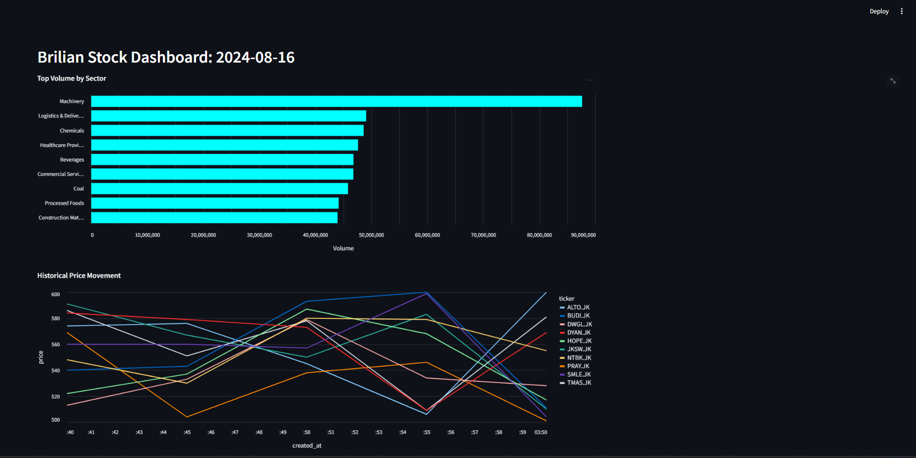
Visualizing Data into Streamlit
In this final section of the lab, we will dive into the analytical aspect by performing insightful query on the aggregated transactional data stored in the MySQL database. Additionally, we will create a simple (near) real-time dashboard to visualize the our data. By combining analytics and visualization, we can easily explore and interpret the data, enabling us to monitor the performance of the business and make data-driven decisions. We will create our dashboard using Streamlit, which is an open-source Python library to build custom web apps. Streamlit is a great tool for quickly building and sharing data applications, and it is quite straightforward to use due to its extensive documentation and intuitive API. In addition to Streamlit, we will utilize Altair, a powerful visualization library, to create interactive and visually appealing charts within our dashboard.Data Analysis
Now, let’s begin our data analysis. To facilitate the analysis process, we will utilizeview in MySQL.
View is a virtual table that is derived from the result of a query. It does not store any data, but rather, it is a stored query that can be treated as a table.
View is an excellent choice for our needs as they allow us to reuse the same query multiple times without having to rewrite the query each time.
We will create a view named volume_today that contains the total trading volume across different sectors on the current day.
| sector | total_volume |
|---|---|
| Machinery | 86189937 |
| Healthcare Providers | 42701507 |
| Coal | 42613419 |
| Beverages | 40638827 |
| Logistics & Deliveries | 43049845 |
| Construction Materials | 38948489 |
| Commercial Services | 40920640 |
| Chemicals | 43433985 |
| Processed Foods | 40158486 |
Streamlit & Altair
Before we dive in, there are some additional packages that we need to install in your current virtual environment:dashboard.
Inside the dashboard folder, we’ll create a file named app.py which will contain the code for our Streamlit application.
Additionally, we need to create a subfolder within dashboard called .streamlit. This subfolder will house a configuration file named secrets.toml for our Streamlit application.
You can accomplish this either through the user interface or by executing the following commands in your project directory:
secrets.toml file with the credentials required to connect with the database.
secrets.toml
app.py file and add the following lines:
dashboard/app.py
secrets.toml.
Then, we set the page configuration for our Streamlit application, including the layout and the page title shown in the browser tab.
Next, we define a function called get_view_data that takes in the name of a view as an argument and returns the data in the view as a dataframe. We also define
get_raw_data which returns the raw transactional data we store in Cassandra.
ttl argument specifies the duration for which the query results will be cached. Since our microbatch processing interval for the aggregated data is 60 seconds,
we set the ttl to 60 seconds as well, indicating that the query results will be cached for 60 seconds before a new query is executed. On the other hand, the second function executes
a query to retrieve all the data from our transactional table in Cassandra. Feel free to adjust these functions as needed, you can even further optimize them by specifying a WHERE clause to avoid
retrieving all data at once.
- The
alt.Chartfunction creates a base chart object. - The
mark_bar(color=color)indicates that the chart is a bar chart with the specified color. - The
encodefunction is used to specify the x and y axes of the chart:- The
x-axisis mapped to thetotal_volume. The title of the x-axis is set to Volume. - The
y-axisis mapped to thesector. The sort argument is set to ‘-x’ to sort the y-axis in descending order. The title of the y-axis is set to None.
- The
- The properties function is used to specify the height, width and title of the chart.
scale=alt.Scale().
st.header, which includes the current date. This title is positioned at the top of the dashboard.
Afterwards, we can then display the plots based on the order we would like to display by calling st.altair_chart().
Now, let’s run the Streamlit app and see the dashboard in action. Execute the following command in the project directory:
Exercise (10 points)
- Objective: Have more proficiency on Kafka and Streamlit.
- Task: Get as creative as you want and add more tables and visualizations by following the steps we have followed through in this lab.